Welcome back to The Long and the Short—where you get an honest take on trading, something you won’t hear elsewhere.
I’m Sandeep Rao, and in the last two episodes, we talked about trend following—what it is, where the idea comes from, and how to build a simple trend-following system using things like breakouts or moving averages.
Then we discussed the importance of using different timeframes, and what happens if you trade only on the long side versus trading both long and short.
Today, we take this a step forward.

Because while trend following on a single asset works—it also comes with its fair share of drawdowns. So the question is: How do we stay in the trend-following game when the system goes through tough phases?
The answer lies in one word: Diversification across assets . Something Donchian did when he started his fund. Today, we’ll follow his footsteps and try a similar experiment across Nifty and Gold.
Alright then—let’s dive in!
Harry Markowitz: The Science of Diversification
In the world of finance, when we talk about diversification, we have to pay homage to Harry Markowitz —the first person to put numbers and mathematical structure behind the idea. Before him, diversification was just common sense advice. After him, it became a science.
Incidentally, both Donchian and Markowitz had remarkably similar early lives. They grew up working in their parents’ shops—Donchian in a rug store, Markowitz in a small family grocery. Maybe it was this exposure to how unpredictable day-to-day business can be that shaped their thinking about risk and uncertainty.
But let’s get back to our business.
Portfolio Selection (1952)
In his 1952 paper “Portfolio Selection,” Markowitz wrote something that gets to the very heart of diversification. He said:
“The adequacy of diversification is not thought by investors to depend solely on the number of different securities held. A portfolio with sixty different railway securities, for example, would not be as well diversified as the same size portfolio with some railroad, some public utility, mining, various sorts of manufacturing, etc. The reason is that it is generally more likely for firms within the same industry to do poorly at the same time than for firms in dissimilar industries.”
What he’s saying is simple yet profound: Owning more things is not diversification. Owning things that behave differently is.
And this idea doesn’t just apply to different industries within the stock market. It extends naturally to different asset classes—equities, bonds, gold, commodities, real estate, and so on.
So while there is some benefit in diversifying within equities—meaning owning 10 stocks instead of 2—the real power of diversification comes from holding multiple assets that are not highly correlated with one another . That is what actually smooths the ride.
Understanding Covariance and Correlation
At this point, I want to introduce two fundamental concepts from statistics that are important to understand in the context of diversification.
The two concepts are: covariance and correlation . These may sound technical, but the ideas are actually quite intuitive. Let’s start with what problem these concepts were originally created to solve.
The Backstory: Galton and Pearson
As always, a bit of a backstory. In episode 5, I spoke about how Galton came up with the idea of “Regression towards the mean.” To understand how strongly parents’ and children’s heights were related, Galton needed a way to measure how two variables move together.
This is where his student Karl Pearson steps in. He formalized Galton’s insight into a mathematical expression—what we now call the Pearson’s correlation coefficient (PCC) .
Covariance: Direction of Relationship
Covariance simply measures the direction of the relationship between two variables.
- If both move up and down together, the covariance is positive
- If one tends to go up while the other goes down, covariance is negative
- If their movements seem unrelated, covariance is near zero
So covariance tells us whether two things tend to move together—but here’s the catch: the actual number is hard to interpret . Because the value of covariance depends on:
- The scale of the data (rupees vs dollars)
- The units used
- The timeframe measured
Change the units, and the covariance number changes.
So while covariance is conceptually useful, practically it’s messy. And that is exactly why Pearson took it one step further and came up with the concept of Correlation .
Correlation: Standardized Covariance
Correlation is simply covariance that has been standardized. It takes that messy covariance number and rescales it into a range between -1 and +1 .
- +1 means move together perfectly
- 0 means no meaningful relationship
- -1 means move exactly opposite
With the standardization, the relationship becomes: clear, comparable, and easy to interpret .
NIFTY and GOLD: Almost Uncorrelated
For example, the correlation coefficient between the long-only trend-following strategies on NIFTY and GOLD is only about 0.04 .
So they are almost uncorrelated.
We’ll take a closer look at this when we go through the backtest results in detail.
Which means both strategies behave quite independently of each other—and this is exactly the kind of relationship Markowitz talked about in his work on portfolio diversification.
This is one of the key reasons why pairing NIFTY with GOLD makes sense—you get diversification benefits. And the other reason, of course, is that we as Indians don’t need a reason to buy gold!
The Backtest Setup
Now let’s get to the interesting parts—the backtests.
Disclaimer: This is not a recommendation to trade, invest, or take positions based on the examples shown. The backtests and simulations discussed here are strictly for educational and illustrative purposes only.
Data and Tools
For this analysis:
- Nifty prices are based on spot data
- Gold is based on GoldM futures with back-adjusted data to create a continuous price series
- These strategies were backtested using TradingView’s strategy testing tools
- The performance summaries were further analyzed using ChatGPT and Claude
I know many of you have asked for a detailed walkthrough on how we build and test strategies. That video is on my list—and I will make it soon.
But for now, let’s stay focused on the Nifty + Gold trend-following framework and see how it behaves.
Strategy Rules
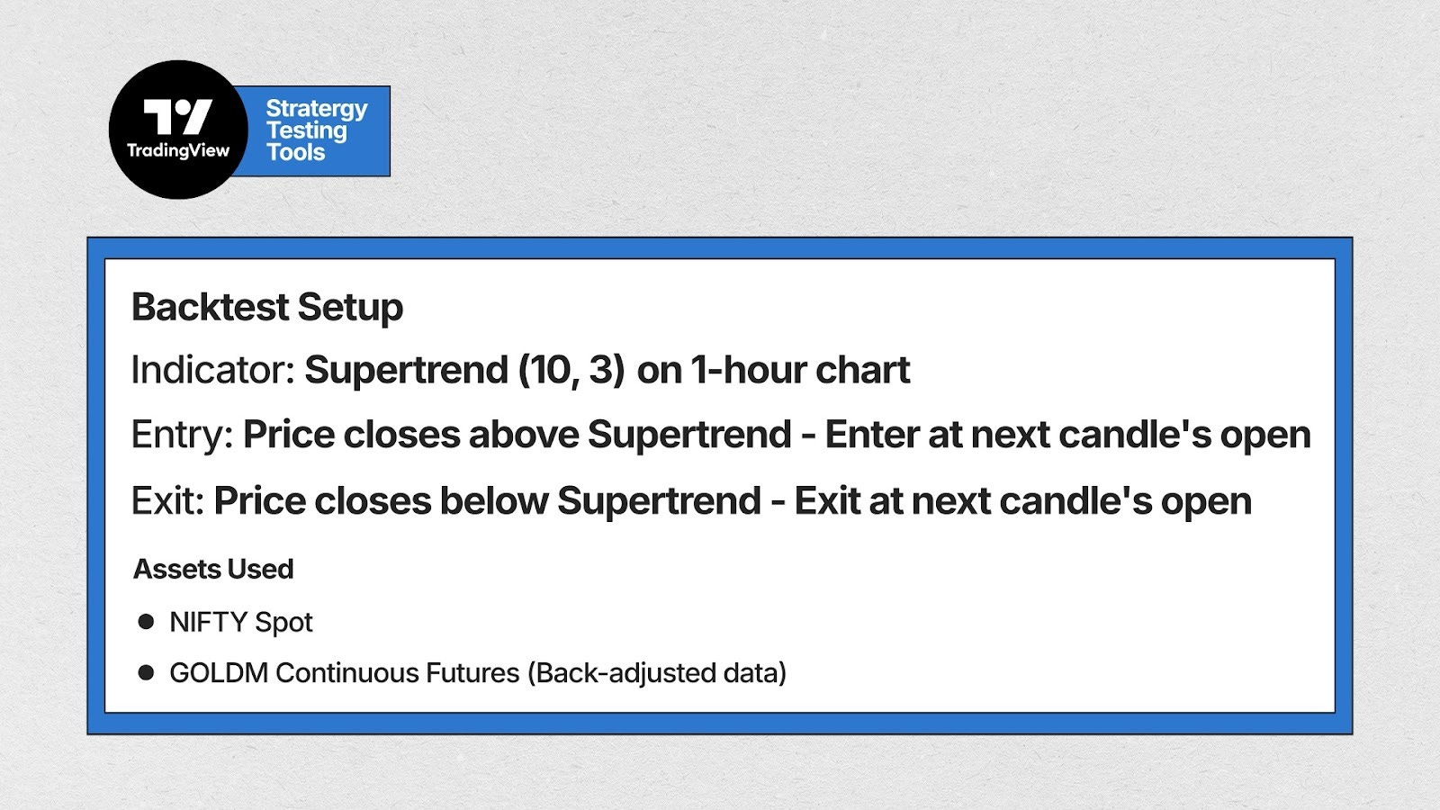
Here are the exact rules used to construct a simple, baseline trend-following system:
Indicator: Supertrend, 10/3 setting
Timeframe: 1-hour chart for both Nifty and GoldM (In the previous episode, we saw the 1-hour performed better than higher timeframes for this style)
Direction: This is a long-only strategy for both assets
Entry Rule: When the price closes above the Supertrend, enter at the next candle’s open
Stop Loss / Exit Rule: The lower Supertrend band acts as the stop loss. When the price closes below the Supertrend, exit at the next candle’s open and wait for the next long setup.
Calculating Returns
I have taken each trade and calculated the percentage return based on the closing price of the asset.
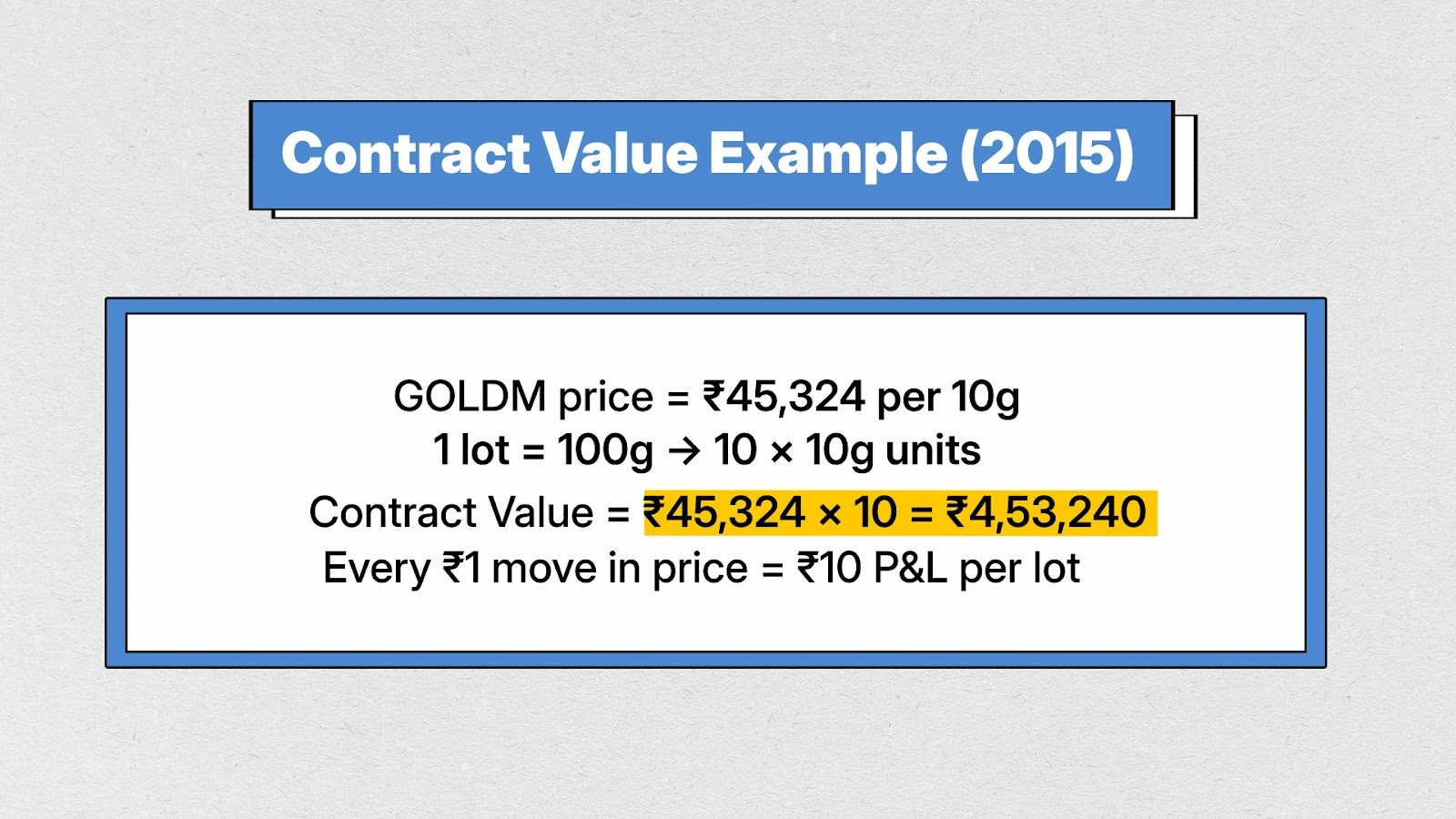
For example: In 2015, GOLDM was quoted at ₹45,324 per 10g. Since one GOLDM lot represents 100g, we multiply by 10 to get the contract value (₹45,324 × 10 = ₹4,53,240).
If the profit on a trade is ₹3,250, then the percentage return is:
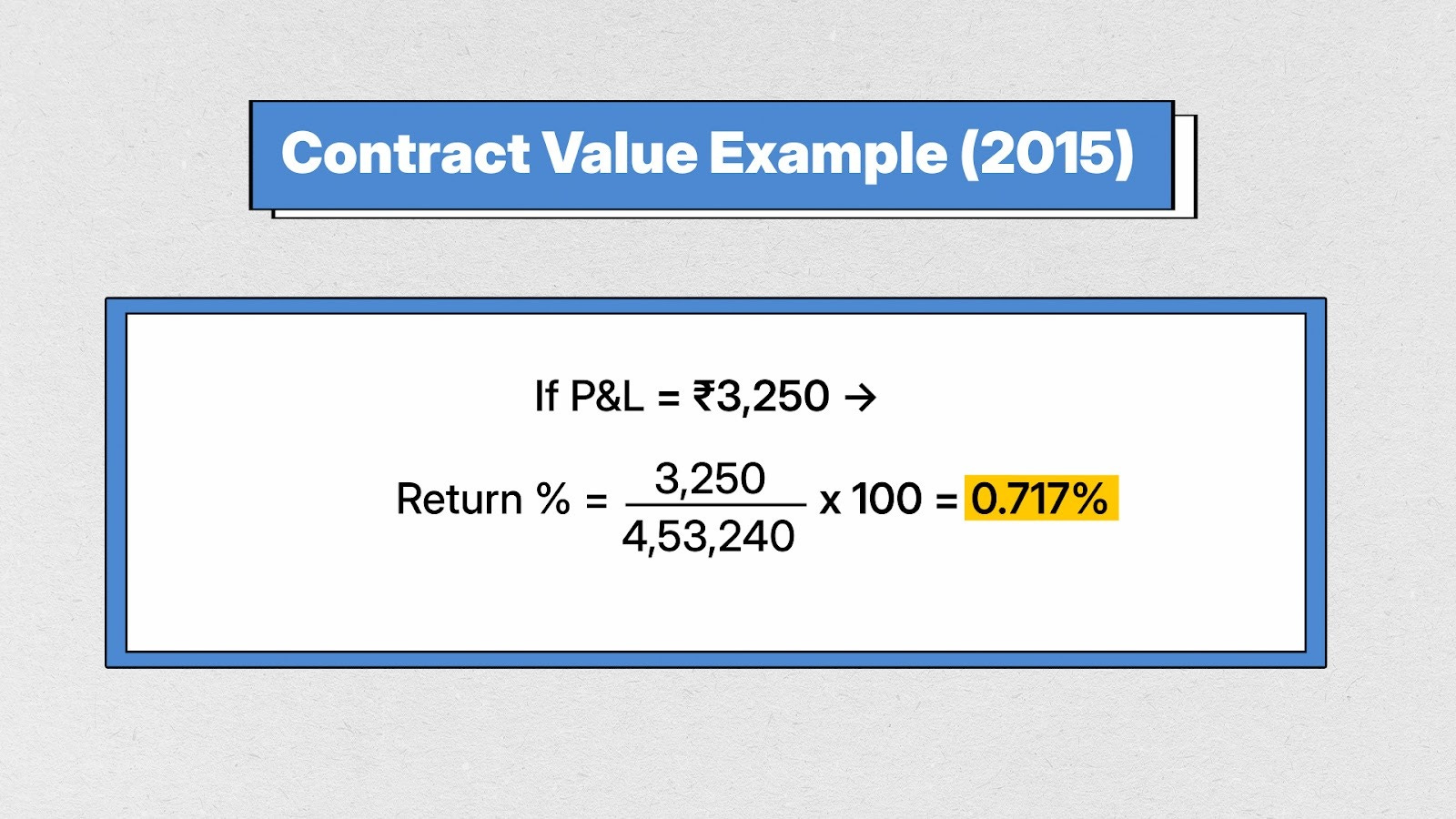
Return % = (3,250 ÷ 4,53,240) × 100 = 0.717%
A similar approach is followed for NIFTY, using the current futures lot size of 75.
Then all percentage returns are added to get a cumulative percentage equity curve for both GOLDM and NIFTY.
This ensures that returns for both instruments are at par and comparable. A leverage factor can be applied later if needed.
To be absolutely clear: We take only long trades in both Nifty and Gold. No shorting. No hedging. We simply follow the long-side trend when it appears.
The Results: Equity Curves
Let’s start with the equity curves. Look at the Cumulative Returns % chart for NIFTY, GOLDM, and the 50:50 Portfolio Strategy.
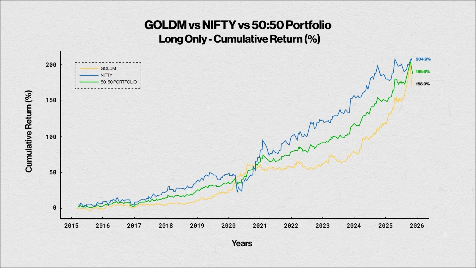
As you can see, over the last 11 years, running this trend-following strategy on GOLDM has delivered about 169% absolute return , whereas on NIFTY it has delivered around 205% .
The 50:50 Portfolio
So the natural question is: What happens if we combine them? Do we get the growth of NIFTY along with the stability of GOLD?
If we look at the equity curve for the 50:50 portfolio, the returns come out to 187% . This is lower than just NIFTY, but higher than just GOLD. So in terms of returns, it sits right in the middle—which is expected.
The Real Story: Drawdown
But the real story here is not the returns. It’s the drawdown.
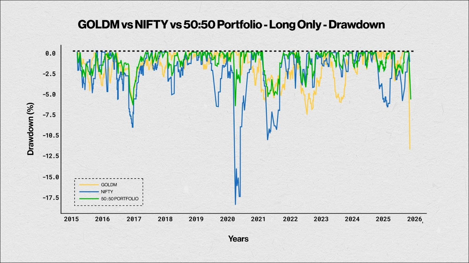
The combined strategy had a maximum drawdown of just 6.6% , compared to 18.5% in NIFTY and 11.8% in GOLD.
This is where the combination really shines—you’re giving up a bit of return, but in exchange, you’re getting much smoother performance and significantly lower stress.
And in real-world trading, lower drawdown is often worth more than higher returns .
Year-Wise Returns: The Yin-Yang Effect
Let me show you a stacked bar chart which will tell us the year-wise returns of each strategy.
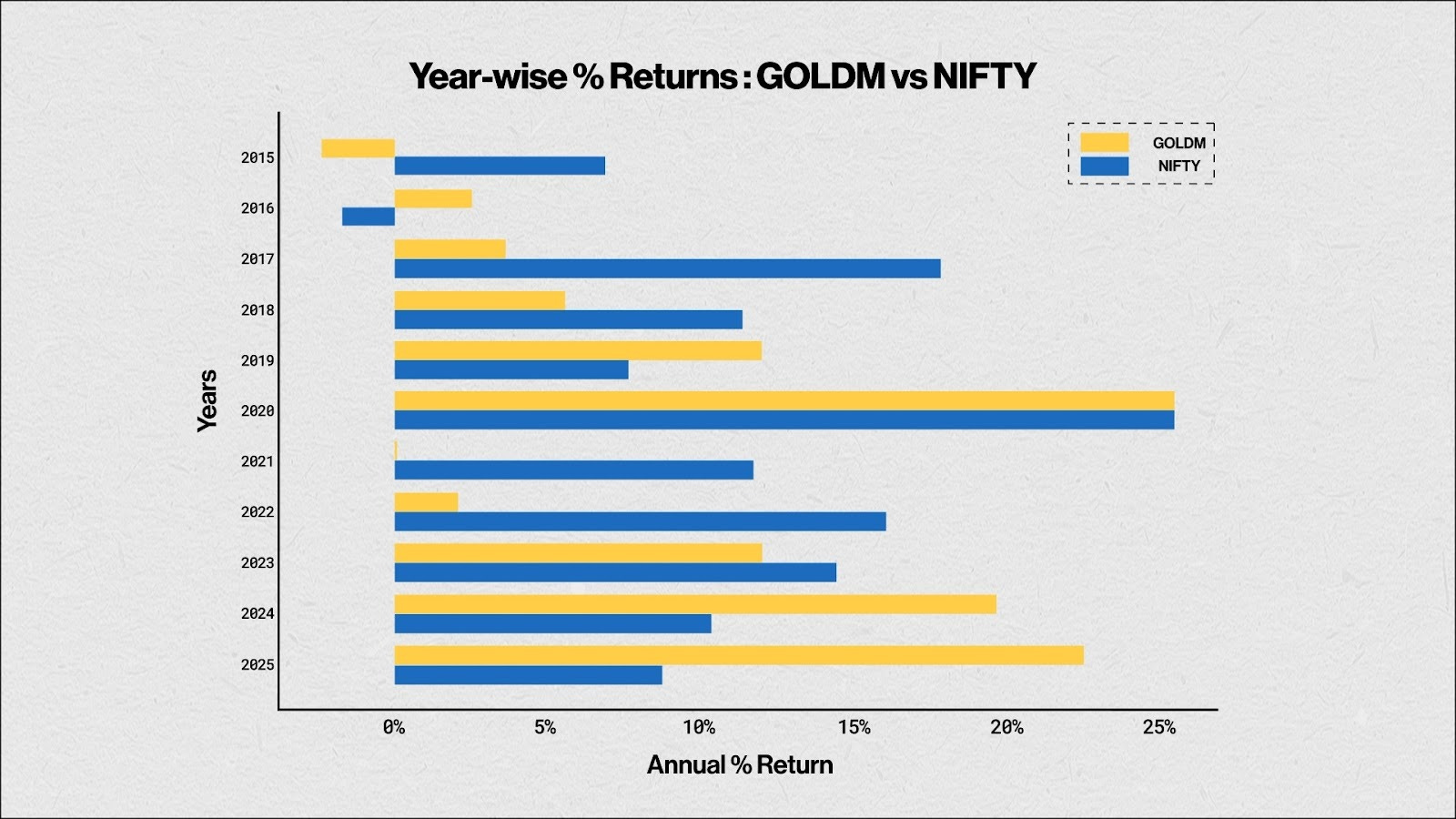
If you look at 2015 and 2016 , you can clearly see an inverse correlation between NIFTY and GOLD. And even beyond those years, the yin-yang kind of movement continues. When one trends up, the other often slows down or consolidates. The cyclical nature of these trends becomes particularly visible in the returns.
This is exactly why combining NIFTY and GOLD tends to hit a sweet spot.
You’re not betting on just one side of the market—you’re allowing one asset to balance the other.
And there’s another advantage, especially for us in India: Gold often acts as a hedge against rupee depreciation . So when the rupee weakens, gold prices typically go up, offering an additional layer of protection to the portfolio.
Key Performance Metrics
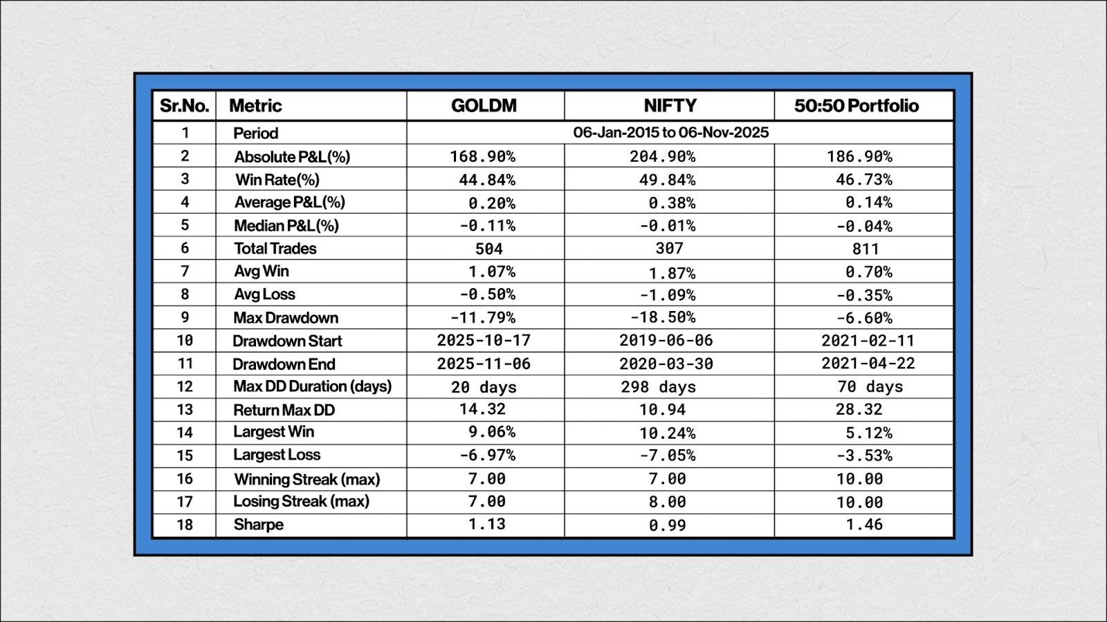
Now, moving to the other key performance metrics:
As we already saw, the returns and drawdowns individually are different—but when we combine them in the 50:50 portfolio, the number of trades naturally increases. However, what really stands out is the Return-to-Max Drawdown ratio , which is the best in the 50:50 case, coming in at 28.32 .
This is a very strong efficiency metric because it tells us how much return we’re getting for every unit of drawdown risk taken.
Also, notice the maximum drawdown duration —which is the time it takes to recover from the worst drawdown—is only 70 days in the 50:50 portfolio compared to Nifty. That’s quite reasonable and definitely easier to handle psychologically compared to longer recovery periods.
The Sharpe ratio is also higher in the 50:50 portfolio. This essentially confirms that when you combine two uncorrelated strategies, you improve your risk-adjusted returns.
Correlation Analysis
Which brings us to the next piece we spoke about earlier: correlation. So let’s now look at the correlation between these three strategies and understand how they move relative to each other.
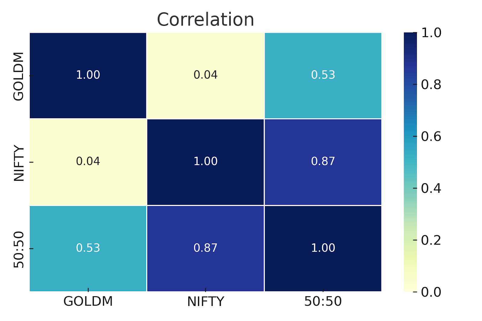
GOLDM and NIFTY long-only strategies are almost uncorrelated (~0.04) , which means they are excellent diversifiers.
Though the 50:50 portfolio is moderately correlated to GOLDM (~0.53) and highly correlated to NIFTY (~0.87)—and that’s because NIFTY has more directional movement.
This lack of correlation in the two strategies is exactly why the portfolio’s drawdowns are shallower.
Buy and Hold Comparison
The other thing that we need to do is to compare the buy & hold performance of these assets: GOLDM returned about 161% and NIFTY returned about 214% .
Now, you may ask—”Sandeep Uncle, all this is fine… but if buy and hold gives almost the same returns, then why trade at all?”
The Answer: Look at the Drawdowns
NIFTY saw a 38% drawdown, and GOLDM saw around 21% drawdown .
So even if the headline returns of the strategies look somewhat comparable with buy and hold, the risk-adjusted returns tell a different story .
A trading or systematic approach gives much better stability than pure buy and hold in this case. Also, in trading, you can use leverage. More on that later.
Post-2020 Performance
I also spoke about returns post-2020, so let’s look at the cumulative returns percentage and drawdown curves from 2020 up to November 2025.
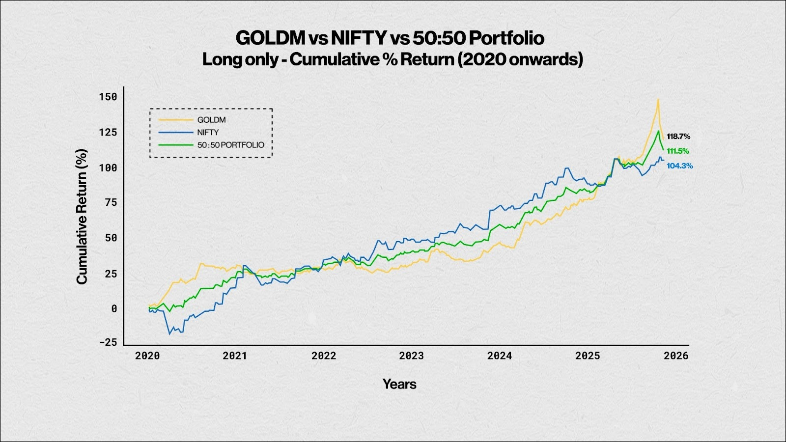
As expected, Gold has outperformed recently, so it looks stronger in the more recent part of the chart. But it’s important to note that until mid-2025, Gold was actually trailing NIFTY. So if you only look at recent performance, it can give a slightly misleading picture.
This is exactly why trading both together makes sense.
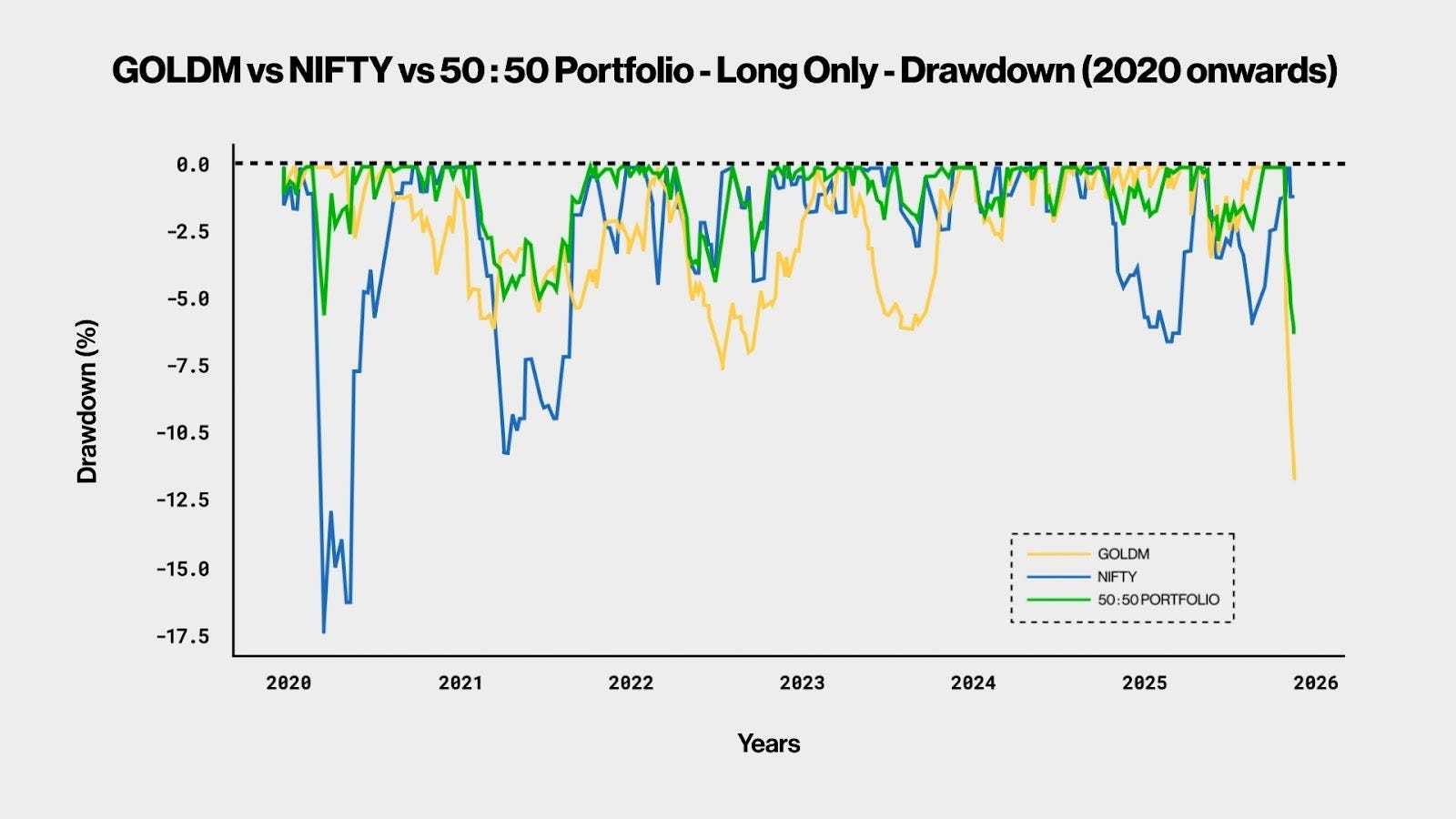
Drawdown Comparison
And you can see this again in the drawdown curve. NIFTY alone had a deep drawdown of around 17% in March 2020.
But when we combine NIFTY + GOLD, the maximum drawdown is only around 6% , and that drawdown is actually more recent.
So the key takeaway here is: The combination smooths the equity curve and reduces the depth of drawdowns, which is extremely valuable from a psychological and risk-management perspective.
Understanding Leverage
At this point, I want to talk about leverage and its effects and why this backtest is designed the way it is—without leverage or compounding factored in.
On a side note: I spoke about leverage as a concept in the video I made on Margin vs. Leverage—I’ll link that in the description, so you can check it out if you haven’t already.
Why No Leverage in the Backtest?
Now, an important thing: all the numbers I showed earlier are calculated without leverage .
There are different ways to backtest a strategy. Some people start with a fixed capital, then keep adding profits, and calculate returns based on that. I have not done that here.
Why? Because in 2015, NIFTY was around 8,500, and today it’s around 25,700. Over the last 10 years, margins and lot sizes have changed multiple times. So, if I were to maintain one fixed leverage multiplier, the first step is to calculate everything without leverage—which is exactly what I’ve done. For simplicity, I’ve also kept the lot size fixed at 75.
Calculating Leverage
Now, if someone is comfortable taking 2x leverage , that’s possible too:
For NIFTY: At today’s contract value, you could keep around 9.5 lakhs per lot , even though the exchange margin required is only around 2.2 lakhs. Which means the exchange is effectively offering 9x leverage, but you are choosing to operate at 2x.
For GOLDM: The contract value is about 12.5 lakhs, so at 2x leverage, you would keep around 6.25 lakhs per lot , even though the exchange margin is only around 1.25 lakhs.
So, for a 50:50 portfolio—1 lot NIFTY + 1 lot GOLDM —your capital requirement at 2x leverage would be around 15.75 lakhs , even though the combined exchange margin requirement is only around 3.45 lakhs.
The Leverage Trade-Off
Do note that—when you increase leverage, say 2x, returns double, but drawdowns also double . So the leverage multiplier is a personal decision, based on your risk tolerance. There is no single rule that works for everyone.
That’s why I have presented backtest results without leverage and without compounding, instead of assuming a starting capital and adding profits along the way. It keeps the results clean, comparable, and unbiased.
Wrapping Up the Trend-Following Series
In short, in this three-part series on trend following, we looked at:
- Part 1: What is trend following
- Part 2: Ways and methods of identifying trends and creating a system to capture trends
- Part 3: An example of a diversified trend-following system and how to think about leverage
Closing Thoughts
And that brings me to the end of this 3-part series on Trend Following. I hope you found these ideas useful.
If you have any questions about this episode, drop them in the comments—I’ll do my best to answer them.
And yes, don’t forget to subscribe to the channel. See you in the next episode of The Long & The Short Show.
Till then—trade safe, and stay curious.